This article walks through the complete statistical profile of Baccarat – expected value, variance, and standard deviation for Player, Banker, and Tie – with step-by-step calculations, dispersion tables across different sample sizes, and a direct comparison with roulette. If you need to know how Baccarat behaves mathematically from a single hand to a hundred thousand, everything is here.
Expected Value, Variance, and Standard Deviation of Baccarat Bets
Baccarat offers three primary wagers: Player, Banker, and Tie. The expected value, variance, and standard deviation for each bet are calculated using standard discrete probability formulas.
Expected Value – the average result per hand over the long run. Each possible outcome is multiplied by its probability, then all products are summed. This single number tells the casino how much it earns (or the player loses) per unit wagered, on average:
iv>
Completeness condition – the probabilities of all possible outcomes must add up to 1 (absolute certainty that something happens). If they don’t, the model is broken:
Variance – measures how far actual results tend to scatter from the expected value. Each outcome’s deviation from the mean is squared (so negative and positive swings don’t cancel each other out) and weighted by its probability. A higher variance means wilder swings:
Standard Deviation – the square root of variance. Squaring the deviations in the variance formula inflates the units, so taking the root brings them back to the same scale as the original bet. This is the number used to build confidence bands around expected value – the ±2σ and ±3σ ranges you’ll see in the tables below:
Applying these formulas to each of the three Baccarat bets produces the following:
| Bet | EV (M(X)) | Variance (D(X)) | Std Dev (SD(X)) |
|---|---|---|---|
| Banker | 0.0105791 | 0.86002 | 0.9273720 |
| Player | 0.0123508 | 0.90469 | 0.9511527 |
| Tie | 0.143596 | 6.97421 | 2.6408726 |
Banker Bet Breakdown
| Outcome | Payout (x) | Probability (p) | xp | x²p |
|---|---|---|---|---|
| Banker wins | 0.95 | 0.4585974 | 0.4356675 | 0.41388415 |
| Player wins | −1 | 0.4462466 | −0.4462466 | 0.4462466 |
| Tie | 0 | 0.095156 | 0 | 0 |
| Totals | 1 | −0.0105791 | 0.86013075 |
This gives us EV = 0.0105791, D = 0.86002, and SD = 0.92737.
Player Bet Breakdown
| Outcome | Payout (x) | Probability (p) | xp | x²p |
|---|---|---|---|---|
| Banker wins | −1 | 0.4585974 | −0.4585974 | 0.4585974 |
| Player wins | 1 | 0.4462466 | 0.4462466 | 0.4462466 |
| Tie | 0 | 0.095156 | 0 | 0 |
| Totals | 1 | −0.0123508 | 0.904844 |
This gives us EV = 0.0123508, D = 0.9046915, and SD = 0.9511527. The Player bet pays 1:1 with no commission, which makes the payout structure simpler than Banker – but the slightly higher probability of a Banker win means the Player bet carries a marginally larger house edge.
Tie Bet Breakdown
| Outcome | Payout (x) | Probability (p) | xp | x²p |
|---|---|---|---|---|
| Banker wins | −1 | 0.4585974 | −0.4585974 | 0.4585974 |
| Player wins | −1 | 0.4462466 | −0.4462466 | 0.4462466 |
| Tie | 8 | 0.095156 | 0.761248 | 6.089984 |
| Totals | 1 | −0.143596 | 6.994828 |
This gives us EV = 0.143596, D = 6.97421, and SD = 2.64087. The Tie bet is in a different league entirely. Its house edge is roughly 14 times larger than Banker’s, and its standard deviation is nearly three times higher. The 8:1 payout creates occasional large wins that mask a steep long-term cost – making it by far the most volatile and least favorable of the three wagers.
How Results Spread Over Time: The Banker Bet
Absolute Values
| Hands (N) | SD | EV−3σ | EV−2σ | EV | EV+2σ | EV+3σ |
|---|---|---|---|---|---|---|
| 1 | 0.93 | −2.77 | −1.84 | 0.01053 | 1.87 | 2.79 |
| 100 | 9 | −26.77 | −17.49 | 1.053 | 20 | 29 |
| 1,000 | 29 | −77.4 | −48.1 | 11 | 69 | 99 |
| 10,000 | 93 | −173 | −80 | 105 | 291 | 384 |
| 32,000 | 166 | −161 | 5 | 337 | 669 | 835 |
| 70,000 | 245 | 1 | 246 | 737 | 1,228 | 1,473 |
| 100,000 | 293 | 173 | 466 | 1,053 | 1,640 | 1,933 |
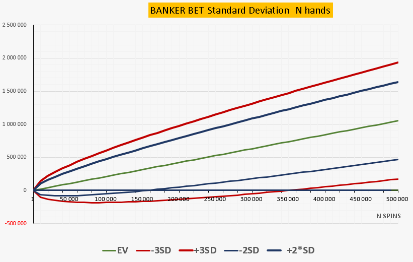
As the number of hands increases, expected value grows in direct proportion to the number of hands played: EV = Wager × N × 0.01053. Standard deviation, however, grows only in proportion to the square root of N: SD = SD₁ × √N, where SD₁ is the standard deviation of a single hand. The ±3σ band captures 99.73% of all actual outcomes, while the ±2σ band captures 95.45%.
Relative Values (Percentage of Total Wagered)
| Hands (N) | SD (%) | EV−3σ | EV−2σ | EV (%) | EV+2σ | EV+3σ |
|---|---|---|---|---|---|---|
| 1 | 92.735% | −277% | −184% | 1.053% | 187% | 279% |
| 100 | 9.273% | −26.8% | −17.5% | 1.053% | 19.6% | 28.9% |
| 1,000 | 2.933% | −7.745% | −4.81% | 1.053% | 6.92% | 9.85% |
| 10,000 | 0.927% | −1.729% | −0.80% | 1.053% | 2.91% | 3.84% |
| 32,000 | 0.518% | −0.502% | 0.016% | 1.053% | 2.09% | 2.61% |
| 70,000 | 0.351% | 0.001% | 0.352% | 1.053% | 1.75% | 2.11% |
| 100,000 | 0.293% | 0.173% | 0.466% | 1.053% | 1.64% | 1.93% |
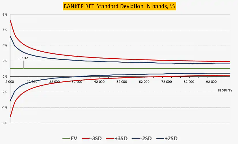
In absolute terms, EV outpaces SD over time. In relative terms, the house edge per hand stays fixed at 1.053% regardless of bet size or the number of hands played. What changes is the spread: as N grows, standard deviation as a percentage shrinks and converges toward EV. In practice, this means that the longer the game continues, the tighter actual results cluster around the mathematical expectation.
Short-Run Risk vs. Long-Run Certainty
The EV and SD charts for the Banker bet illustrate a fundamental truth about casino mathematics: even though the house always has a positive expected result, actual outcomes can dip below zero in the short run – meaning the casino can and does lose over small samples. The Tie bet, meanwhile, is far more volatile than either Player or Banker, which are roughly similar in both expected value and standard deviation.
Over a longer horizon, the picture changes. Banker bet results land entirely in positive territory starting around 32,000 hands at the 95.45% confidence level (±2σ), and from about 70,000 hands at 99.73% confidence (±3σ).
Standard deviation is ultimately a measure of risk. It lets you calculate the range of likely outcomes around the expected value for any number of hands and any chosen confidence level. To put concrete numbers on it: a casino spreading a $1,000 Banker bet over 1,000 hands can expect, with 99.73% confidence, a result somewhere between −$77,446 and +$98,506, and with 95.45% confidence, between −$48,121 and +$69,181. The same $1,000 bet over 100,000 hands narrows the 99.73% confidence range to an entirely positive window: +$173,240 to +$1,932,760.
Baccarat vs. Roulette: A Comparison of Dispersion Behavior
It is worth comparing Baccarat’s Player bet with roulette’s even-money wagers (Red/Black, Odd/Even), since they look similar on the surface. Both pay 1:1, and their single-hand standard deviations are nearly identical (SD_Player = 0.95113 versus SD_Red = 0.99964). Equal standard deviations mean equal-sized dispersion bands – yet the bands behave quite differently.
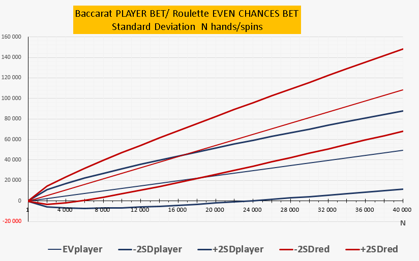
On roulette, the spread of actual results enters positive territory much earlier – around 5,472 spins – compared to 23,535 hands for the Baccarat Player bet. The reason is the gap in expected value: roulette’s house edge is a steady 2.7%, while Baccarat’s Player bet carries only 1.25%. On a chart, EV determines the slope of the central line and the entire dispersion envelope around it. Because Baccarat’s EV line has a shallower angle, its dispersion band takes longer to clear the zero axis. In other words, the casino’s actual results on Baccarat take significantly longer to settle into reliably profitable territory.
Practical Applications
Understanding variance and standard deviation is essential for several areas of casino operations: calculating loss-based discounts and rebates, structuring junket programs, setting VIP betting limits, determining cash reserve requirements, and assessing overall risk exposure.
Because of its low house edge and low variance, Baccarat is also the game most commonly chosen by online casino players looking to clear wagering requirements on bonuses.